Contextual Analysis In Sport Using Tracking Networks

Javier Martin Buldu is an expert on the analysis of non-linear systems and the understanding of how complex systems organise themselves, adapt and evolve. He focuses on the application of network science and complex systems theory in the analysis of sports. Buldu’s work is based on the principle that teams are far more than the simple aggregation of their individual players. By collaborating with organisations such as the Centre of Biomedical Technology in Madrid, La Liga, ESADE Business School, IFISC research institute and the ARAID Foundation, he has been able to combine elements of graph theory, non-linear dynamics, statistical physics, big data and neuroscience to construct various networks using positional tracking data of a football match. These networks are then able to explain what happens on the pitch beyond conventional ways of assessing the performance of individual players to understand team behaviours.

What Is Complex System Theory?

A complex system is a system composed by different parts that are connected and interact with one another. This system has properties and behaviours that cannot be explained by simply breaking down the system into its individual parts and analysing each individual part independently. For example, the human brain is a complex system and it has proven extremely challenging for scientists to fully understand how it performs all its functions, from how memory is stored to how cognition appears and disappears during certain illnesses. On the other hand, the human brain’s most fundamental component, the neuron, has been thoroughly studied and documented by science. Scientists have been able to recreate models and simulations of neuron behaviour, understand their shape and how they communicate with other neurons. However, this robust understanding of single neuron behaviour has not been sufficient to allow scientist to comprehend the interplay and interdependencies of the 80 billions neurons that form the human brain and that allows it to perform all of its complex behaviours. Instead, in order to appropriately study the brain, scientist need to pay attention to entire human cognitive system as a whole.

The idea behind complex systems like the human brain is what Buldu wanted to introduce in the analysis of football. While it is interesting to have information about isolated player performance, such as the number of shots, passes or successful dribbles, it is also important to understand the context in which these events take place. Additional insights on the performance of players and teams can be obtained by analysing information about how a player interacted with his teammates and the opposition’s players. Paying attention to individual player performances and aggregating those together is not enough to fully understand how a team behaves during a match.

Instead, a complex system approach to football analysis would, for example, look at the link created between two or more players when they pass the ball between them. A network of these players can then be created by simply leveraging event data collected from notational video analysis to count the number of passes from player A to player B and vice versa. These types of passing networks are increasingly common in football match analysis and team reports, as they clearly illustrate information about how a team played during a match, where its players were most frequently located on the pitch and how they interacted with each other.

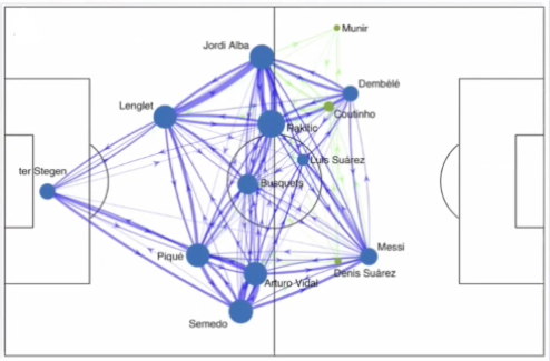
Passing Network between FC Barcelona players (Source: Javier Martin Buldu at FC Barcelona Sports Tomorrow)

However, more complex and informative networks can be developed by leveraging positional tracking data instead of event data. While event data is generated through notational analysis by tagging specific actions, positional tracking data instead describes the position of the 22 players and the ball on the pitch at any moment in time during a match of football. Unfortunately, positional tracking data is challenging to access for most analysts. That is why Buldu collaborated with La Liga to obtain a positional tracking dataset containing Spanish football league matches. To capture this information, La Liga uses Mediacoach, a software that acquires the positional coordinates of players and the ball using a TRACAB optical video tracking system that requires the installations of specialised cameras across the football stadiums. Mediacoach’s system allows them to track a player’s position at 25 frames per second and a precision of 10cm. Thanks to this detailed tracking dataset received from La Liga, Buldu was able to explore the different interactions between players to construct a number of complex tracking networks in football. 

Proximity Networks

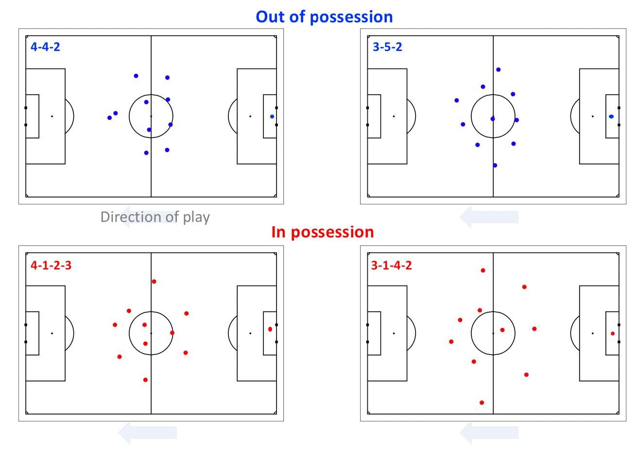
The first network that Buldu produced explored the proximity between players on the pitch. He first calculated an arbitrary 360 degrees distance around a player, let’s say a 5m radius, and used it as a threshold to identify any other players that may fall inside that particular player’s area. If another player was located inside of the first player’s surrounding area, a link was then created between those two players. If those two players were from the same team, a positive link was created, while if they were from opposing teams a negative link was assigned to that interaction instead. By increasing or decreasing the radius of the distance surrounding each player (i.e. 5m, 10m or 15m radius), Buldu produced different networks and links between players following this method.

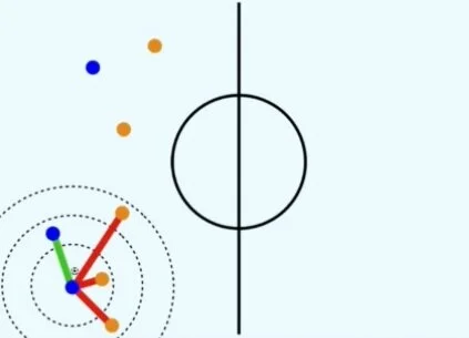
Proximity radius at 5m, 10m and 15m showing links with players of the same team (green) and with opposing players (red) (Source: Javier Martin Buldu at FC Barcelona Sports Tomorrow)

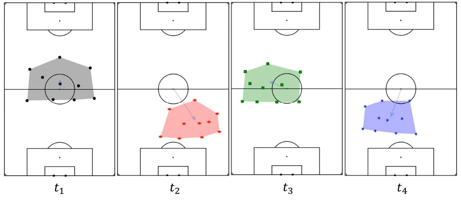
The challenge of producing a variety of proximity networks is that they may prove difficult to analyse, as the links identified in a single video frame using a 5m radius around each player may be very different to those found using a 15m radius. On top of that, the analysis should look at how those proximity networks evolve over a number of frames during the match. In order to gather practical insights from these networks, Buldu aimed to study the number of positive and negative links for each of the teams, as well as the organisation of the proximity network structure, its temporal evolution and how they change in relation to the zone of the pitch and the various phases of the game.

Proximity analysis of the 3-player links for all players in a match between Atletico Madrid and Real Valladolid (Source: Javier Martin Buldu at FC Barcelona Sports Tomorrow)

He first counted the number of links between three different players forming a triangle. He then classified each triangle into two categories: positive (all players from the same team) or mixed triangles (at least one player from the opposing team). Buldu was then able to determine which team had dominance over the other at different times of the match by then counting the number of positive triangles and the number of mixed triangles produced with a certain threshold distance. The team with the the highest proportion of positive triangles (i.e. all three players in close proximity to each other forming a triangle were from the same team) was deemed to have been dominant over its opposition.

Marking Networks

The second type of network that Buldu was able to construct with positional tracking data was the time a player was covering an opposing player during a defensive phase of play. Again, by setting an arbitrary threshold distance around a defender, a link between the defender and opposing player can be set by counting the time both players are in close proximity to one another. This process produces a matrix that illustrates the defenders on one of the axis and the attackers on the other axis, and provides a rough idea about the amount of time that each attacking player was being marked and by which defensive player. By interpreting the marking matrix analysts are able to identify the players with the highest accumulated time being marked by a defensive player.

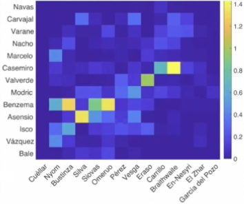
Player marking matrix between Real Madrid (y-axis) and Leganes (x-axis) showing how often each Real Madrid players was marked by a Leganes player (Source: Javier Martin Buldu at FC Barcelona Sports Tomorrow)

Since matrices are the mathematical extraction of a network, this information can be drawn onto a diagram of a football pitch to plot the position of players during defensive actions. The size of each node in this network indicates the time an attacking player was being defended. By using these marking networks, analysts can clearly visualise the interactions and efforts of attacking and defending players during a match of football.

Player marking network between Real Madrid and Leganes (Source: Javier Martin Buldu at FC Barcelona Sports Tomorrow)

Coordination Networks

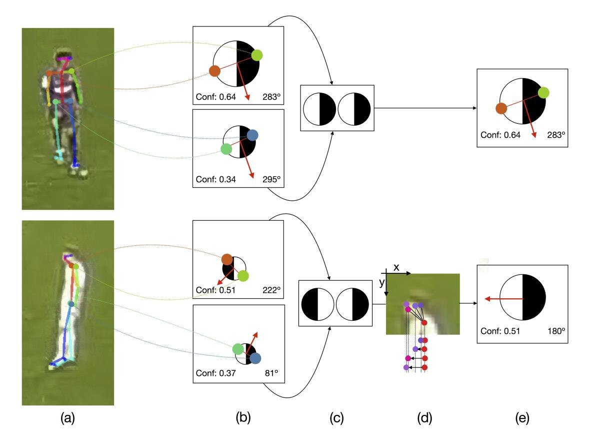
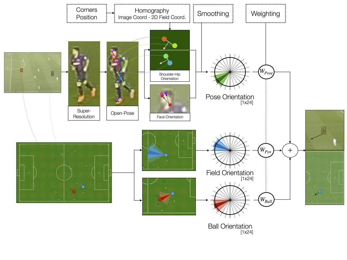
The third network that Buldu produced evaluated the coordination of movements between players of the same team. The network computed the velocity and direction of movement of two players to measure the alignment of their vectors. When this vector alignment was high, a high value link between these two players was created. When the alignment was low, a lower value connection was also derived from the two players’ movements. This method results in a matrix that illustrates how well players are coordinated with their own teammates. Two different matrices can be produced, one to analyse offensive phases of play and one for defensive phases.

Vector alignment of two attacking players (Source: Javier Martin Buldu at FC Barcelona Sports Tomorrow)

Similarly to marking networks, coordination network matrices can also be translated into diagrams on a football pitch, where the nodes represent each player on the pitch while the size of each node indicates the amount of coordination the player has with the rest of his teammates. The links between two nodes also indicate the level of coordination between two particular players of the same team.

Movement coordination of each player with the rest of his teammates (Source: Javier Martin Buldu at FC Barcelona Sports Tomorrow)

This type of analysis, especially when split between offensive and defensive players, can help analysts better understand the level of coordination between attack and defensive plays. For instance, an analyst or coach may want to see high degrees of coordination when the team defends as a block as well as how that coordination changes during the different phases of the game.

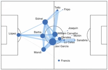
Ball Flow Networks

Lastly, the final network developed by Buldu focused on ball movement between different areas of the pitch. This network was produced by splitting the football pitch into different sections and counting the number of times the ball travelled from one section to another in order to create links between two different sections. This ball flow network can also be visualised on a diagram of a football pitch, with the nodes representing each section of the pitch and links indicating the number of times the ball moved from one section to the next. The size of these nodes indicate the amount of time the ball was being played inside that particular section of the pitch. By constructing an entire ball moving network during a match, analysts can then identify which are the most important sections of the pitch for their teams and assess how to exploit different sections in the opposition’s side in order to create dangerous opportunities.

Ball flow network for a match between FC Barcelona and Espanyol (Source: Javier Martin Buldu at FC Barcelona Sports Tomorrow)

Buldu’s work provides a great analytical framework to assess the complexities of sports in which a large diversity of factors can influence different outcomes of the game. It is crucial that when analysing a sport, all the available contextual information is analysed from various perspectives that can together provide a more complete evaluation of performance. Researchers, scientists and analysts are increasingly producing exciting work with positional tracking data that can open the door to new sophisticated methodologies and models to help coaches better understand the key influential factors of their team’s performance.

Further Reading:

• Futbol y Redes Website

• Buldu, J. M., Busquets, J., & Echegoyen, I. (2019). Defining a historic football team: Using Network Science to analyze Guardiola’s FC Barcelona. Scientific reports, 9(1), 1-14. Link to article.

• Buldu, J. M., Busquets, J., Martínez, J. H., Herrera-Diestra, J. L., Echegoyen, I., Galeano, J., & Luque, J. (2018). Using network science to analyse football passing networks: Dynamics, space, time, and the multilayer nature of the game. Frontiers in psychology, 9, 1900. Link to article.

• Garrido, D., Antequera, D. R., Busquets, J., Del Campo, R. L., Serra, R. R., Vielcazat, S. J., & Buldú, J. M. (2020). Consistency and identifiability of football teams: a network science perspective. Scientific reports, 10(1), 1-10. Link to article.

• Herrera-Diestra, J. L., Echegoyen, I., Martínez, J. H., Garrido, D., Busquets, J., Io, F. S., & Buldú, J. M. (2020). Pitch networks reveal organizational and spatial patterns of Guardiola’s FC Barcelona. Chaos, Solitons & Fractals, 138, 109934. Link to article.

• Martínez, J. H., Garrido, D., Herrera-Diestra, J. L., Busquets, J., Sevilla-Escoboza, R., & Buldú, J. M. (2020). Spatial and Temporal Entropies in the Spanish Football League: A Network Science Perspective. Entropy, 22(2), 172. Link to article.

A New Way Of Classifying Team Formations In Football

One of the most important tactical decisions made in football is deciding on the best team formation,  determining what roles each player has and the playing style. Laurie Shaw and Mark Glickman from the Department of Statistics at Harvard University recently developed an innovative, data-driven way of identifying different tendencies seen by managers when giving tactical instructions to their players, specifically around team formations. They measured and classified 3,976 observations of different spatial configurations of players on the pitch for teams with and without the ball. They then analysed the changes of these formations throughout the course of a match.

 While team formations in football have evolved over the years, they continue to heavily rely on a classification system that simply counts the number of defenders, midfielders and forwards (i.e. 4-3-3). However, Laurie and Mark argued that this system only provides a crude summary of player configurations within a team, ignoring the fluidity and nuances these formations may experience during specific circumstances of a match. For instance, when Jürgen Klopp prepares his formations at Liverpool, he creates a defensive version where all players know their roles and an offensive one that aims to exploit the best areas of the pitch. Therefore, Liverpool prepare different formations for different phases of the game; a detail that is lost when describing them as using a simple 4-3-3 formation.

Identifying Defensive And Offensive Formations

The researchers used tracking data to make multiple observations of team formations in the 100 matches analysed; separating formations with and without possession. By doing so, they identified a unique set of formations that are most frequently used by teams. These groups helped them classify new formation observations to then analyse major tactical transitions during the course of a match.

Source: Shaw, L. & Glickman, M. (2019) Dynamic analysis of team strategy in professional football. Barça Sports Analytics Summit.

The above diagram from Laurie and Mark’s study shows a defending team moving as a coherent block by having players retain their relative position, showing that their formation is not defined by the positions of players on the pitch in absolute terms but by their positions relative to one another. Starting from the player in the densest part of the team, Laurie and Mark calculated the relative position of each player using the average angle and distance between said player and his nearest neighbour over a specific time period in a match, and subsequently repeating the same process with the latter’s neighbor and so on. By calculating the average vectors between all pairs of players in the team, they obtained a center of mass of a team’s formation, which is then aligned to the centre of the pitch when plotting team formations.

Source: Shaw, L. & Glickman, M. (2019) Dynamic analysis of team strategy in professional football. Barça Sports Analytics Summit.

The researchers made multiple observations of a team’s defensive and offensive configurations throughout the match. They aggregated together the observed possession into two-minute intervals. For example, for the team in possession they plotted all possessions into two-minutes time periods and then measured their formations in each of those sets, and did the same process for the team without possession during the same time period.

The diagram below shows a set of formation observations for a team during a single match, illustrating that the team defends with a 4-1-4-1 formation, but attacks with three forwards and with the fullbacks aligning with the defensive midfielder. These findings also illustrate that while the defensive players remained compacted, the movement of attacking players, such as central striker was more varied. The consistency in all the observations also suggest that the managers did not change formations significantly during the match. 

Source: Shaw, L. & Glickman, M. (2019) Dynamic analysis of team strategy in professional football. Barça Sports Analytics Summit.

Grouping Similar Formations Together Into Five Clusters

Additionally, Laurie and Mark used an agglomerative hierarchical clustering to identify unique sets of formations that teams used in the 100 matches analysed; constituting 1,988 observations of defensive formations and 1,988 observations of offensive ones. To be able to group formations together, they first had to define a metric that established the level of similarity between two separate formations. The similarity between two players in two different formations is quantified using the Wasserstein distance, using their two bivariate normal distributions, with their own means and covariance matrix, where the Wassertein distance between them is calculated by squaring the L2 norm of the difference between their means. However, an entire team’s formation consists on a set of 10 bivariate normal distributions, one for each outfield player. Therefore, to compare two different team formations the researchers calculated the minimum cost of moving from one distribution to another using the total Wasserstein distance. The blue area in the diagram below indicates the number of players that deviate from the formation’s average position.

Laurie and Mark also found that two formations may be identical in shape, but one may be more compact than the other. In order to classify formations solely by shape and not by their degree of expansion across the pitch, they had to scale the formations so that compactness is no longer a discriminator in their clustering.

Once this was resolved, the hierarchical clustering applied to the dataset simply found two most similar formation observations based on the Wasserstein distance metric to combine them and form a group. Then, it found the next two most similar ones, forming more groups, and so on. This process identified 5 groups of formations with each group containing 4 variant formations, producing a total of 20 unique formations.

Source: Shaw, L. & Glickman, M. (2019) Dynamic analysis of team strategy in professional football. Barça Sports Analytics Summit.

 The first group of formations correspond to 17% of all observations in the sample of Laurie and Mark’s study. The commonality of these four variants in the first group of formations is that there are five defenders, but with variations in the number of midfielders and forwards. This group of formations was most predominant in defensive situations, with between 73%-88% of their observations being of teams without possession.

Source: Shaw, L. & Glickman, M. (2019) Dynamic analysis of team strategy in professional football. Barça Sports Analytics Summit.

Group 2 and Group 3 share the commonality of having 4 defenders, with group two in the second row consisting of more compact midfields, as oppose to a more expanded midfield in Group 3 formations.

Source: Shaw, L. & Glickman, M. (2019) Dynamic analysis of team strategy in professional football. Barça Sports Analytics Summit.

Group 4 contained predominantly attacking formations consisting on three defenders, where the wingbacks push high up the pitch, and with variations in structure of the midfield and forward line.

Source: Shaw, L. & Glickman, M. (2019) Dynamic analysis of team strategy in professional football. Barça Sports Analytics Summit.

Group 5 formations contained two defenders with fullbacks pushed up the field and with some variations in the forward line with either two or three forwards, as well as different structures on the midfield. These group of formations consistent entirely in offensive formations observations.

As illustrated by these groupings, the hierarchical clustering Laurie and Mark applied was very efficient in separating offensive and defensive formation observations, even after excluding the dimension of the area of the formation (i.e. how compact the formations are) as a discriminator. Additionally, while some of these formations aligned with traditional ways to describe formations, such as 4-4-2 or 4-1-4-1, others do not clearly fall within these historical classifications. Once the formation clusters were identified, the researchers developed a basic model selection algorithm to categorise any new formation observations into any of these groups by finding the maximum likelihood cluster.

Transitions Between Offensive And Defensive Formations

Laurie and Mark took their research a step forward by evaluating the pairing tendencies by coaches of the various defensive and offensive formations. In the diagram below, they illustrated that the teams that defend with Cluster 2 frequently transition into an offensive formation like the one in Cluster 16, with the wingbacks pushing up. Also, half of the teams with the defensive formation in Cluster 9 tend to use the offensive formation in Cluster 10, while the other half transition to a formation similar to Cluster 18. This demonstrated a clear story in to how a player transitions from their defensive role to their attacking role. Moreover, it showed that some defensive formations allow more variety in terms of the offensive formations than others.

Source: Shaw, L. & Glickman, M. (2019) Dynamic analysis of team strategy in professional football. Barça Sports Analytics Summit.

Tactical Match Analysis Through This Methodology

The methodology developed by Laurie and Mark allows teams to measure and detect significant changes in formations throughout the match. They were able to produce diagrams such as the one below to illustrate the formation changes in both defensive (diamonds) and offensive (circles), including annotations of goals (top lines) and substitutions (bottom lines). The story of the match in the diagram shows a red team conceding a goal in the first half and then making a significant tactical change at half time as well as a substitution. Laurie and Mark found this situation very usual, as whenever there was a major tactical change it was often accompany with a substitution. Comparing with other matches, they found that this particular red team made major tactical changes at half time in around a quarter of their matches, providing insights into how their manager reacts to given situations.

Source: Shaw, L. & Glickman, M. (2019) Dynamic analysis of team strategy in professional football. Barça Sports Analytics Summit.

In another diagram, they demonstrated how their methodology can also help study how changes in formation begin impact the outcome of a match. In this match, the blue team were predominantly attacking down the wings in the first half, with most of their high quality opportunities coming from right wing. In the second half, the red team changed their formation to five defenders instead of four, which reduced the attacks from the blue team’s right wing and instead going through the centre, presumably less busy since they now have two midfielders rather than three.

Source: Shaw, L. & Glickman, M. (2019) Dynamic analysis of team strategy in professional football. Barça Sports Analytics Summit.

Finally, this methodology also allows teams to establish the link between chance creation and formation structure. They can also measure how different the position of opposing players is from their preferred defensive structure (i.e. how are are they out of position). At the same time, it allows for the measurement of the level of attacking threat by assessing the amount of high value territory the attacking team controls near the defending team’s goal. These pitch control models enable the measurement of threatening positions even when no shot took place. Laurie and Mark suggest that this kind of analysis allows teams to better understand how the attacking team maneuvers defenders out of their positions or how they take advantage defending team being out of position after a high press or a counterattack.

Citations:

• Shaw, L. & Glickman, M. (2019) Dynamic analysis of team strategy in professional football. Barça Sports Analytics Summit. Link to paper

Automated Tracking Of Body Positioning Using Match Footage

A team of imaging processing experts from the Universitat Pompeu Fabra in Barcelona have recently developed a technique that identifies a player’s body orientation on the field within a time series simply by using video feeds of a match of football. Adrià Arbués-Sangüesa, Gloria Haro, Coloma Ballester and Adrián Martín (2019) leveraged computer vision and deep learning techniques to develop three vector probabilities that, when combined, estimated the orientation of a player’s upper-torso using his shoulder and hips positioning, field view and ball position.

This group of researchers argue that due to the evolution of football orientation has become increasingly important to adapt to the increasing pace of the game. Previously, players often benefited from sufficient time on the ball to control, look up and pass. Now, a player needs to orientate their body prior to controlling the ball in order to reduce the time it takes him to perform the next pass. Adrià and his team defined orientation as the direction in which the upper body is facing, derived by the area edging from the two shoulders and the two hips. Due to their dynamic and independent movement, legs, arms and face were excluded from this definition.  

To produce this orientation estimate, they first calculated different estimates of orientation based on three different factors: pose orientation (using OpenPose and super-resolution for image enhancing), field orientation (the field view of a player relative to their position on the field) and ball position (effect of ball position on orientation of a player). These three estimates were combined together by applying different weightings and produce the final overall body orientation of a player.

1. Body Orientation Calculated From Pose

The researchers used the open source library of OpenPose. This library allows you to input a frame and retrieve a human skeleton drawn over an image of a person within that frame. It can detect up to 25 body parts per person, such as elbows, shoulders and knees, and specify the level of confidence in identifying such parts. It can also provide additional data points such as heat maps and directions.

However, unlike in a closeup video of a person, in sports events like a match of football players can appear in very small portions of the frame, even in full HD frames like broadcasting frames. Adrià and team solved this issue by upscaling the image through super-resolution, an algorithmic method to image resolution by extracting details from similar images in a sequence to reconstruct other frames. In their case, the researcher team applied a Residual Dense Network model to improve the image quality of faraway players. This deep learning image enhancement technique helped researchers preserve some image quality and detect the player’s faces through OpenPose thanks to the clearer images. They were then able to detect additional points of the player’s body and accurately define the upper-torso position using the points of the shoulders and hips.

Source: Arbues-Sangüesa, A.; Haro, G.; Ballester C. & Martin A. (2019) Head, Shoulders, Hip and Ball... Hip and Ball! Using Pose Data to Leverage Football Player Orientation. Barça Sports Analytics Summit.

Once the issue with image quality was solved by researchers and the player’s pose data was then extracted through OpenPose, the orientation in which a player was facing was derived by using the angle of the vector extracted from the centre point of the upper-torse (shoulders and hips area). OpenPose provided the coordinates of both shoulders and both hips, indicating the position of these specific points in a player’s body relative to each other. From these 2D vectors, researchers could determine whether a player was facing right or left using the x and y axis of the shoulder and hips coordinates. For example, if the angle of the shoulders shown in OpenPose is 283 degrees with a confidence of 0.64, while the angle of the hips is 295 degrees with a confidence level of 0.34, researchers will use the shoulders’ angle to estimate the orientation of the player due to its higher confidence level. In cases where a player is standing parallel to the camera and the angles of either the hips or the shoulders are impossible to establish as they are all within the same coordinate in the frame, then researchers used the facial features (nose, eyes and ears) as a reference to a player’s orientation, using the neck as the x axis.

Source: Arbues-Sangüesa, A.; Haro, G.; Ballester C. & Martin A. (2019) Head, Shoulders, Hip and Ball... Hip and Ball! Using Pose Data to Leverage Football Player Orientation. Barça Sports Analytics Summit.

This player and ball 2D information was then projected into the football pitch footage showing players from the top to see their direction. Using the four corners of the pitch, researchers could reconstruct a 2D pitch positioning that allowed them to match pixels from the footage of the match to the coordinates derived from OpenPose. Therefore, they were now able to clearly observe whether a player in the footage was going left or right as derived by their model’s pose results.

Source: Arbues-Sangüesa, A.; Haro, G.; Ballester C. & Martin A. (2019) Head, Shoulders, Hip and Ball... Hip and Ball! Using Pose Data to Leverage Football Player Orientation. Barça Sports Analytics Summit.

In order to achieve the right level of accuracy in exchange for precision, researchers clustered similar angles to create a total of 24 different orientation groups (i.e. 0-15 degree, 15-30 degrees and so on), as there was not much difference in having a player face an angle of 0 degrees or 5 degrees.

 2. Body Orientation Calculated From Field View Of A Player

Researchers then quantified field orientation of a player by setting the player’s field of view during a match to around 225 degrees. This value was only used as a backup value in case of everything else fails, since it was a least effective method to derive orientation as the one previously described. The player’s field of view was transformed into probability vectors with values similar to the ones with pose orientation that are based on y coordinates. For example, a right back on the side of the pitch will have its field of view reduced to about 90 degrees, as he is very unlikely to be looking outside of the pitch.

Source: Arbues-Sangüesa, A.; Haro, G.; Ballester C. & Martin A. (2019) Head, Shoulders, Hip and Ball... Hip and Ball! Using Pose Data to Leverage Football Player Orientation. Barça Sports Analytics Summit.

3. Orientation Calculated From Ball Positioning

The third estimation of player orientation was related to the position of the ball on the pitch. This assumed that players are affected by their relative position in relation to the ball, where players closer to the ball are more strongly oriented towards it while the orientation of players further away from it may be less impacted by the ball position. This step of player orientation based on ball position accounts for the relative effect of ball position. Each player is not only allocated a particular angle in relation to the ball but also a specific distance to it, which is converted into probability vectors.

Source: Arbues-Sangüesa, A.; Haro, G.; Ballester C. & Martin A. (2019) Head, Shoulders, Hip and Ball... Hip and Ball! Using Pose Data to Leverage Football Player Orientation. Barça Sports Analytics Summit.

Combination Of All The Three Estimates Into A Single Vector

Adrià and the research team contextualized these results by combining all three estimates into as single vector by applying different weights to each metric. For instance, they found that field of view corresponded to a very small proportion of the orientation probability than the other two metrics. The sum of all the weighted multiplications and vectors from the three estimates will correspond to the final player orientation, the final angle of the player. By following the same process for each player and drawing their orientation onto the image of the field, player movements can be tracked during the duration of the match while the remain on frame.

In terms of the accuracy of the method, this method managed to detect at least 89% of all required body parts for players through OpenPose, with the left and right orientation rate achieving a 92% accuracy rate when compared with sensor data. The initial weighting of the overall orientation became 0.5 for pose, 0.15 for field of view and <0.5 for ball position, suggesting the pose data is the highest predictor of body orientation. Also, field of view was the least accurate one with an average error of 59 degrees and could be excluded altogether. Ball orientation performs well in estimating orientation but pose orientation is a stronger predictor in relation to the degree of error. However, the combination of all three outperforms the individual estimates.

Some limitations the researchers found in their approach is the varying camera angles and video quality available by club or even within teams of the same club. For example, matches from youth teams had poor quality footage and camera angles making it impossible for OpenPose to detect players at certain times, even when on screen.  

Source: Arbues-Sangüesa, A.; Haro, G.; Ballester C. & Martin A. (2019) Head, Shoulders, Hip and Ball... Hip and Ball! Using Pose Data to Leverage Football Player Orientation. Barça Sports Analytics Summit.

Finally, Adrià et al. suggest that video analysts could greatly benefir from this automated orientation detection capability when analyzing match footage by having directional arrows printed on the frame that facilitate the identification of cases where orientation can be critical to develop a player or a particular play. The highly visual aspect of the solution makes is very easily understood by players when presenting them with information about their body positioning during match play, for both first team and the development of youth players. This metric could also be incorporated into the calculation of the conditional probability of scoring a goal in various game situations, such as its inclusion during modeling of Expected Goals. Ultimately, these innovative advances in automatic data collection can relief many Performance Analyst from hours of manual coding of footage when tracking match events.

Citations:

Arbues-Sangüesa, A.; Haro, G.; Ballester C. & Martin A. (2019) Head, Shoulders, Hip and Ball... Hip and Ball! Using Pose Data to Leverage Football Player Orientation. Barça Sports Analytics Summit. Link to article.

What are Expected Goals (xG)?

What are Expected Goals (xG)?

Expected Goals, or xG, are the number of goals a player or team should have scored when considering the number and type of chances they had in a match. It is a way of using statistics to provide an objective view to common commentaries such as: ”He shouldn't miss that!” "He's got to score those chances!" "He should have had a hat-trick!”

Goals in football are rare events, with just over 2.5 goals scored on average per game. Therefore, the historical number of goals does not provide a large enough sample to predict the outcome of a match. This means that shots on target and total number of shots are now being used as the next closest stats to predict number of goals. However, not all shots have the same likelihood of ending up in the back of the net.

This is where xG comes into play. Expected Goals uses various characteristics of the shots being taken together with historical data of such types of shots to predict the likelihood of a specific shot being scored. Since xG is simply an averaged probability of a shot being scored, a team or player may outperform or underperform their xG value. This means that they could be scoring chances that the average player would miss or that they could be missing chances that are often scored.

xG is often used to analyse various scenarios:

• To predict the score of an upcoming match using historical data of the teams involved.

• Assess a team’s or player’s “true” performance on a match or season, regardless of their short-term form or one-off actions on a pitch. It provides a data point on the number and quality of chances being created regardless of the final result.

• Identify performing players in underperforming teams, or those who receive less playing minutes, by assessing which ones are more effective than the quality of their chances they receive would suggest.

• Understand the defensive performance of a team by assessing how effectively are they preventing the opponent team from scoring their chances.

Origin of the ExpectedGoals Model

In April 2012, Advanced Data Analyst Sam Green from sport statistics company Opta first explained his innovative approach to assessing the performance of Premier League goalscorers, inspired by similar models being used in American sports. However, it was not until the beginning of the 2017/18 season when BBC’s Match of The Day debut their use of xG by their popular football pundits to make xG a focal topic of conversation by many football fans. 

Over the years, Opta has collected numerous data points of in-game actions in all of the top football leagues. When creating the xG model, Sam Green and the Opta team analysed more than 300,000 shots and a number of different variables using Opta’s on-ball event data, such as angle of the shot, assist type, shot location, the in-game situation, the proximity of opposition defenders and distance from goal. They were then able to assign an xG value, usually as a percentage, to every goal attempt and determine how good a particular type of chance is. As new matches are played new data is collected to continuously refine the xG model.

There is no one specific model to calculate xG. When looking at xG it is important to consider that the xG value would depend on the factors that the analyst creating the xG model wants to incorporate in the calculations. Since its release to the public, the xG theory raised considerable attention in the analytics community, with many enthusiasts working and adjusting the model in their own ways in an attempt to perfect it. This means there are now several different xG models out there, each of them considering different factors. Some would consider whether it was a goal scored with their feet or with their head, other consider the situation that led to the shot and so on, but the final prediction each model outputs have shown to only vary slightly across different models.

How is xG calculated?

Opta’s xG model is based on the fact that the most basic requirement to score goals is to take shots. However, not all strikers score goals from the same number of shots. As Sam Green identified, in the 2011/12 season Van Persie only needed 5.4 shots to score a goal, while Luis Suarez took 13.8 shots for each goal he scored. However, they both shot the same number of times per game they played.

This is why Opta decided to look deeper into the quality of chances each striker received by adding the average location from which each shots was taken. However, they soon realized that location on its own was not enough. A penalty spot chance could come from a penalty kick, a header from a corner or a 1 on 1 against the goalkeeper, each with a very different likelihood of ending up in a goal. That is why Opta decided to incorporate additional data points to the model. Unfortunately, the exact model with all the factors considered by Opta has not been made public but a number of analyst have attempted to replicate or improve the model since its first release.

The xG model was designed to return an xG value for each player, team or chance depending on the dimension that the data is being analysed in: a full season, a particular match, a specific half in a game or group of goal attempts. Let’s say a player like Harry Kane takes 100 shots from chances that, based on historical Premier League data, have a probability of being scored of 0.202 (or 20.2%). Kane's xG value would be 20 expected goals scored (100 shots x 0.202). This xG number would contain an average of some ‘big scoring chances’ Kane took, such as penalties with 0.783xG, other non-penalty shots inside the box with varying xG values such as 0.387xG and maybe even shots outside the box with an 0.036xG value. The models attempts to balance the number of shots a player takes with the quality of these chances. For example, a player may get himself into very dangerous attacking positions inside the box in 23 occasions with high xG value and score the same number of goals than a player that continuously tries his luck from outside the box with 81 shots attempts that have a lower xG value.

Once an xG value has been calculated, a player or team’s performance can be evaluated on whether they are over or under-performing such value. In the above example, Harry Kane may actually score 25 goals during the full season, 5 goals above his 20 xG value, suggesting that his ability of converting chances is above-average and he can find the net in difficult scoring situations. Similarly, a player with a 20 xG value who has scored 15 goals suggests that he is missing chances that he probably should have scored.

Opta took xG a step further and assessed the impact the player had to a specific chance using their shot quality. They did so by factoring into the xG calculation the propensity to hit the target a shot taken by the player has and then comparing the former xG(Overall) value against this new xG(On Target) one. Their analysis showed that at the time Van der Vaart’s shooting saw his xG increase from 6.9xG to 10.3xG(On Target), suggesting that the type of shots he took were of higher quality than the average when xG was calculated before he took the shot. xG(OT) when compared to actual goals may also indicate how much a player was affected by the quality of goalkeeping he had to face. In the same season, Mikel Arteta scored 7 goals with just 3.5xG(OT) suggesting he got ‘luckier’ in front of goal as his shooting quality should have only given him just over 3 goals.

xG(OT) can be used to assess goalkeeping quality when used in reverse. Since it only takes into consideration shots on target, a keeper’s participation in these sort of chances is crucial to the final outcome of the play. De Gea conceding 22 goals with an 27xG(OT) suggests that he has blocked goals in situation were they are normally conceded.

Why are Expected Goals important in today's football?

Luck and randomness influences results in football more often than any other sports. We have all seem teams being dominated throughout a match and manage to score a last minute winning goal while having a lower number of chances than their opposition. But how sustainable is that? We have also seen world class strikers become out-of-form and spend a few games without seeing the back of the net. Is the player not taking advantage of the chances being provided by his teammates? xG allows us to assess the process over the results of a match, or performance of a player or team, by rating the quality of chances instead of the actual outcome.

The most used example to explain xG’s efficiency is the Juventus season of 2015/16. Juventus only won 3 out of their first 10 games but the difference between their actual goals and xG was considerably high. This meant that the had the chances but were not converting them, suggesting that their negative run of results might not last if they just get a bit luckier in front of goal. Sacking manager Massimo Allegri could have been a mistake, since after match day 12 their luck changed and ended up winning the league title with 9 games spare.

xG gives us a more accurate way of predicting match outcomes than by simply using individual stats. In the Premier League, only 71.6% of teams that had the most shots won the fixture, while close to 81% of teams that obtain a higher xG score win games. It eliminates historical assumptions that popular tradition in football has created and provides a statistically relevant point of argument to whether the performance of a player or team is above or below the average given a number of historical data points.

When using expected goals to see which players are hitting the target more or less than the numbers suggest they should, teams can scout promising prolific goalscorers if they consistently score more goals than the quality of chances they get. On the other hand if a player surpasses his expected goals for a few games but has no history of doing so in the past, it might come down to his form and luck rather than goalscoring talent, and he might struggle to sustain that over a long period of time.

Limitations of the Expected Goals model

The xG model is only as good as the factors being input into its calculations. These data inputs are limited by the data we possess today from companies such as Opta. Other factors, such as shot power, curl or dip on the shot or whether the goalkeeper is unsighted or off balance might not be considered in most xG models out there. Due to model being based on averages, the random nature of a football match and the rarity of goals in the sport makes it almost impossible to consider with enough statistical significance all historical factors that can cause a goal to be scored. xG should be used as indicative and supportive information for decision making purposes and generating opinions rather than a finite answer to the performance of a team or player.

As the model’s creator Sam Green puts it: “a system like this will also fail to predict a high scoring game. Since it is based on averages and with around half of matches featuring fewer than 2.5 goals, this is to be expected”. We also need to consider that a shot taken by a Manchester United striker should have a higher xG than one taken by a Stoke City player, suggesting that on average Man Utd would outperform their xG on a chance by chance basis while Stoke City would underperform it if the xG is calculated using averages from all English teams' shot history.

Criticism and the Future of xG models

The recent misuse of Expected Goals as a analysis metric during pundit commentary has encouraged numerous criticism. A team may score one or two difficult chances early in a game and sit back for the remaining of the 90 minutes, allowing their opponents to take many shots from different positions, thus increasing the opponents xG. One could then claim that the losing team achieved a higher xG therefore deserves the win. This is why xG should always be taken with additional context of the game before creating a verdict. Statistics can just tell us what happened in a game but a wider view is necessary to show you how it happened and give you a clearer idea on what’s yet to come. Certain in-game actions by players cannot be measured with a statistical model today, such as the ability of a defender in getting in front of a shot attempt despite never touching the ball.

There is also a strong resistance from the football community to the use of data. Football is a traditional and emotional sport by nature, with experience and accepted wisdom dominating people’s opinions. Most fans see the use of statistics as intrusive and challenging their popular and historic knowledge of “the beautiful game”. After experiencing their team lose, most of them are not interested in listening to television pundits discuss how their team performed against their expected goals. Despite analytics having plenty to offer to football performance analysis, there are still doubters. xG’s debut in Match of the Day shaked social media with instant mentions of “stat nerds” and claims that the numbers in football are “pointless” and “bollocks”. However, it has been made clear by Opta that xG is not intended to ever replace scouts and pundits but simply aid them in their analysis of a game.

Despite all this resistance and criticism by some pundits and football fans to accept this new era of football analysis, Opta and various sport analysts continue to evolve the use of statistics to analyse performance in numerous areas in football. Models such as xG are the first round of statistical systems and will soon be followed by upcoming ones such as Defensive Coverage, which will assess tackles, blocks, interceptions, man-marking and clearances. Football’s data revolution has started and will continue to see developments every season.